Finding Shortest Paths in Hexagonal Torus Topologies

Numerous people working on packet routing in SpiNNaker have been faced with the problem of generating shortest paths in the hexagonal mesh and torus topologies of SpiNNaker networks. This article introduces the (widely known) method for calculating shortest paths in hexagonal meshes. For hexagonal toruses topologies, the solution is less obvious. Though a number of solutions have been produced, this article describes a new, cleaner method which is able to generate all possible routes unlike existing solutions. Finally, we conclude with a proof-of-principle Python implementation which demonstrates the technique.

Minimal Paths in Hexagonal Meshes

As a first step lets look at a hexagonal mesh topology:

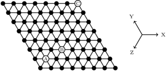
There are three axes in a hexagonal topology meaning we can define positions or distances using vectors with three components.

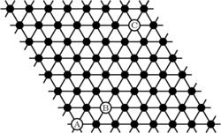
For example the vectors for the labelled nodes A, B and C could be written:

• $\mathbf{a} = (1,1,0)$
• $\mathbf{b} = (3,2,0)$
• $\mathbf{b} = (7,7,0)$

Position vectors of two points can be subtracted to get the vector between those two points as usual. For example, the vector from A to B could be written:

$\mathbf{b} - \mathbf{a} = (3,2,0) - (1,1,0) = (2, 1, 0)$

This vector can in turn be converted into a path by taking a number of steps along the hexagonal axes in turn as defined by the vector. These steps need not necessarily be taken in order, for example given our example vector the following paths could be taken:

• +Y, +X, +X
• +X, +Y, +X
• +X, +X, +Y

In practice, one of the following two schemes are widely used. In 'Dimension Order Routing' the steps for each dimension are carried out in a fixed sequence, for example all X steps followed by all Y steps followed by all Z steps. In 'Longest Dimension First Routing', the dimensions are traversed in descending order of the number of steps required. No matter the route taken, however, the length of the vector (and thus the route) is:

$\| (a, b, c) \| = \lvert a \rvert + \lvert b \rvert + \lvert c \rvert$

How about the vector $(3, 2, 1)$? This vector also gets us from A to B and takes 6 hops. Something strange is going on: we have multiple vectors from A to B with different lengths! This is very much unlike conventional, non-hexagonal topologies where a vector between two points is uniquely defined. This begs the question: given that multiple vectors exist, which is the smallest between A and B and is it unique?

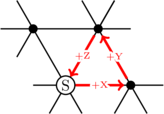
To answer our question, lets look more closely at the hexagonal coordinate system. Unlike most 3D systems, the three dimensions are not orthogonal (i.e. at right-angles). This means that any hop along an axis also moves us slightly on the other axes. For example, moving positively along the Z axis also moves us slightly negatively on the X and Y axes.

For a particularly dramatic demonstration of the phenomenon see the vector $(1,1,1)$. The figure below illustrates the dimension order route of this vector starting from S and terminating back at S.

Given that we know the vector $(1,1,1)$ does not move anywhere, we must therefore be able to freely add and subtract it from any other vector without altering where that vector points. For example, lets try our original vector from A to B:

$(2,1,0) - (1,1,1) = (1, 0, -1)$

The new vector also takes us from A to B but this vector is only two hops compared with the three it originally took. If we subtract $(1,1,1)$ again, however, the new vector in fact becomes longer again at three hops:

$(1,0,-1) - (1,1,1) = (0, -1, -2)$

In fact, the vector $(1, 0, -1)$ is minimal and unique. To prove this and to demonstrate that a minimal, equivalent vector can be found for any vector, consider the following:

• If a vector has three positive elements, subtracting $(1,1,1)$ reduces the length of the vector by three.
• If a vector has two positive, non-negative elements, subtracting $(1,1,1)$ decreases the magnitude of the two positive elements and increases the magnitude of the remaining element resulting in a net reduction in length of one.
• If a vector has only one positive, non-zero element, subtracting $(1,1,1)$ decreases the magnitude of that element and increases the magnitude of the remaining two resulting in a net increase in length of one.
• Similar arguments about cases with negative, non-zero elements and the addition of $(1,1,1)$ can also be made.

As a result of these rules we can state that:

• A vector with at most one positive, one negative and one zero element is minimal.
• A vector with two or more zero elements is minimal.
• Changes to a minimal vector monotonically increase its length and thus a minimal vector is unique.

Thus, to calculate the minimal form of a hexagonal vector the following function can be used:

$\operatorname{minimiseVector}(a,b,c) = (a,b,c) - [\operatorname{median}(a, b, c) \cdot (1,1,1)]$

To give an example, the minimal form of the vector from B to C can be found like so:

$$\begin{eqnarray} \operatorname{minimiseVector}(\textbf{c} - \textbf{b}) &=& \operatorname{minimiseVector}((4,5,0)) \\ &=& (4,5,0) - [4 \cdot (1,1,1)] \\ &=& (4,5,0) - (4,4,4) \\ &=& (0,1,-4) \end{eqnarray}$$

The careful reader will also notice that this rule implies that a minimal route in a hexagonal topology will travel along at most two dimensions since one element of any minimal vector is always zero.

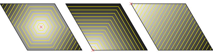
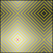
To attempt to aid intuition of distances in hexagonal mesh topologies, the plots below show the distance from a single point (marked by a red cross) in a hexagonal mesh topology. White points are close while black points are distant. Contour lines (yellow) show points of equal distance.

Minimal Paths in Hexagonal Toruses

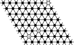
With minimal routes in meshes defined, we aim to extend our definition to a hexagonal torus. To construct a hexagonal torus topology from a hexagonal mesh, roll up the mesh to connect the top-most nodes to the bottom-most nodes to form a tube. Next, bend the left-most end of the tube to connect to right-most end of the tube forming a torus (doughnut). The resulting topology is commonly drawn flat like so (with wrap-around links omitted for clarity):

Hexagons are not square: Failure of the naive approach

Before describing our solution to the problem of finding shortest paths on toruses we will first attempt to demonstrate why the problem may be more difficult than it first appears.

In a conventional (square) torus topology, distances can be found by translating everything such that the source is in the centre of the system. After this transformation, all paths from the source are identical to those in a mesh and thus can be found straight-forwardly.

For example, given a square torus, the distances from the point marked by the red cross can be seen in the figure below:

If the whole system is translated such that distances are measured not from an arbitrary point but from the centre, we get the following:

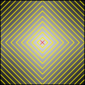
This distance plot is identical to that of a (square) mesh when the source is the centre of the system and therefore the same methods for finding paths apply.

Unfortunately, this solution does not apply to hexagonal toruses. The distance plots from the centre of the system for meshes and toruses are shown below:

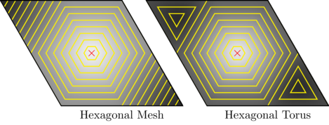
The two are different since in the hexagonal mesh the top-left and bottom-right parts of the system simply get further and further away. In the hexagonal torus, however, we can wrap-around making the very edges of the corners closer than they were. The key fact is that re-centring the system is not a viable approach for hexagonal toruses.

We are aware of two existing correct but slightly clumsy solutions to the problem:

Gollywhomper

This implementation translates the system such that the source is at $(0,0,0)$, $(w/2, h/2, 0)$ and $(w-1,h-1,0)$ and computes the shortest path from each of these as if they were meshes. ($w$ is the width of the system, $h$ is the height of the system) The three solutions are then compared and the smallest chosen.

INSEE/Tickysim

In this implementation, the (four) combinations of wrapping and not wrapping around the X and Y axes are tried. For each of these combinations, three paths are then computed which use only the X-and-Y, Y-and-Z and X-and-Z axes. The shortest of the twelve examined paths is selected.

In the case of Gollywhomper this method is essentially brute-forcing the mesh distance measure into providing a valid solution. The INSEE/Tickysim method is being somewhat more systematic and bears some resemblance to the solution we propose below but test out far more cases than necessary.

Solution

In our solution we first translate all points by $-\mathbf{a}$ such that the source, A, is at $(0,0,0)$:

From here we can make the observation that our path falls into one of the following four categories:

1. Doesn't wrap-around (moves only +X, +Y and -Z)
2. Wraps-around left-to-right only (moves only -X and +Y)
3. Wraps-around bottom-to-top only (moves only +X and -Y)
4. Wraps-around left-to-right and bottom-to-top (moves only -X, -Y and +Z)

Because of the limited set of movements allowed depending on the category we fall into, we can infer more about our routes. As we'll show shortly, we can exploit this knowledge to cheaply compute which of the four categories minimal routes fall into and thus trivially determine a minimal route.

Given:

• $(x, y, 0)$, the coordinates of the destination (after the initial translation)
• $0 \le x < w$
• $0 \le y < h$
• $w \times h$ are the topology's dimensions

The minimal route for each category can be straight-forwardly found in the same way as a route through a mesh:

1. $\operatorname{minimiseVector}(x, y, 0)$
2. $\operatorname{minimiseVector}(-(w-x), y, 0)$
3. $\operatorname{minimiseVector}(x, -(h-y), 0)$
4. $\operatorname{minimiseVector}(-(w-x), -(h-y), 0)$

From these we can in turn calculate their lengths. Thanks to our knowledge of the ranges of values in each of the four cases, the general distance expressions for each category can be heavily simplified:

1. $\operatorname{max}(x, y)$
2. $w-x+y$
3. $x+h-y$
4. $\operatorname{max}(w-x, h-y)$

By evaluating each of these distance expressions we can cheaply determine the categories whose paths are minimal. Given this information, we can then compute a minimal route for that category (and thus the whole torus) as described above.

As an aside, the above distance expressions leads us to a compact expression (which has also been derived independently in graph theoretical studies of hexagonal toruses) for the shortest path length in a hexagonal torus topology between $(0,0,0)$ and $(x,y,0)$:

$$\begin{eqnarray} \operatorname{torusPathLength}((0,0,0), (x, y, 0), w, h) = \operatorname{min} &(& \operatorname{max}(x, y) \\ &,& w-x+y \\ &,& x+h-y \\ &,& \operatorname{max}(w-x, h-y) \\ &)& \end{eqnarray}$$

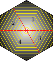
For an additional, graphical way of visualising this technique, a plot of distances from the bottom-left corner (marked with a red cross) is presented. The contour lines (yellow) show equidistant points in the topology. The areas of the hexagonal torus which correspond with each of the four categories are also labelled.

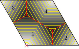
We can re-draw the plot as a hexagon by slicing it up along the boundaries between categories and moving the pieces as if they were wrapping-around the hexagonal axes. This form shows how the contour lines actually continue to grow in a regular, hexagonal fashion: the triangular patterns we have seen in previous plots are simply an artefact of drawing the system as a parallelogram.

Python Implementation

As a proof of principle, a Python implementation of the above shortest-vector calculation for a hexagonal torus topology is given below:

def shortest_vector(src, dst, w, h):
    """Get a shortest path from src to dst in a hexagonal torus with
    dimensions w and h.

    Parameters
    ----------
    src : (x, y, z)
    dst : (x, y, z)
    w : int
    h : int

    Returns
    -------
    A shortest path `(x, y, z)`.
    """
    # Break-appart tuples
    sx, sy, sz = src
    dx, dy, dz = dst

    # Convert to (x,y,0)
    sx, sy, sz = sx-sz, sy-sz, 0
    dx, dy, dz = dx-dz, dy-dz, 0

    # Translate destination by the vector used to translate the source to
    # (0,0,0)
    dx = (dx - sx) % w
    dy = (dy - sy) % h

    #              Distance          Vector
    approaches = [ (max(dx, dy),     (dx, dy))
                 , (w-dx+dy,         (-(w-dx), dy))
                 , (dx+h-dy,         (dx, -(h-dy)))
                 , (max(w-dx, h-dy), (-(w-dx), -(h-dy)))
                 ]

    # Select the best approach.
    distance, (dx, dy) = min(approaches)

    # Return a minimal hexagonal (3D) vector
    vector = (dx, dy, 0)
    median = sorted(vector)[1]
    return (dx-median, dy-median, -median)


if __name__=="__main__":
    # A random example
    print(shortest_vector((1,2,0), (5,6,1), 10, 10))
    # (0, 0, -3)

Generating all possible routes

While the technique described above will generate a shortest path in a hexagonal torus, it does not generate all shortest paths. This is a problem for authors of routing algorithms since not generating all valid routes will result in link use imbalance.

As a first step, we should randomly break ties between categories of equal distance when deciding what route to generate. While this gets us 50% of the way there, there is a problem: minimal vectors within a hexagonal torus are not unique in the general case, unlike minimal vectors in a hexagonal mesh. To demonstrate this, take a look at the example below:

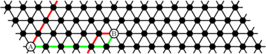
In the example above two minimal paths from A to B are shown:

• $(5,0,-1)$ (in green)
• $(1,0,-5)$ (in red)

Notice that both of these vectors are of length 6 and both are minimal according to the rules previously set out and yet you cannot get from one to the other by adding $(1,1,1)$, thus these are actually different vectors.

A key observation to make here is that spiralling from top-to-bottom makes travelling along the X axis and the Z axis equivalent when travelling multiples of the system's height along the X axis. The complementary observation can be made about travelling along the Y axis in multiples of the width of the system.

Since the minimisation approach described in the article above explicitly avoids wrapping around the torus when it is not necessary, we must modify the solutions generated to (sometimes) spiral along the Z axis.

Considering the case where $\lvert x \rvert$ is greater than or equal to the height of the system, the maximum number of spirals, $N$, is:

$N = \lfloor \frac{x}{h} \rfloor$

Note that since $x$ can be negative $N$ can be too. In this case, the spirals simply travel in the opposite direction.

We can then pick a random number, $n$, between $0$ and $N$ (inclusive) as the number of spirals to introduce. For every $nh$ steps in the Z direction we form a spiral which is equivalent to $nh$ steps along the X axis and so our new vector becomes:

$(x - nh, y, z - nh)$

The process is similar for the introduction of spirals around the Y axis.

Proof that spiral transformation preserves minimality

Notice that the transformation for introducing spirals, described above does not involve adding multiples of $(1,1,1)$ and thus it is not immediately apparent that the result should also be a minimal vector. In the following proof by cases we show that the transformation always produces minimal routes.

Proof is currently a work in progress. Actual implementation indicates that this is true, however.

Python Implementation

The following Python implementation is very similar to the one above but incorporates the changes described in this section and will randomly select minimal vectors to generate.

import random

def shortest_vector_2(src, dst, w, h):
    """Get a random shortest path from src to dst in a hexagonal torus with
    dimensions w and h.

    Parameters
    ----------
    src : (x, y, z)
    dst : (x, y, z)
    w : int
    h : int

    Returns
    -------
    A shortest path `(x, y, z)`, selected randomly from those available (i.e.
    may return different results when called at different times).
    """
    # Break-appart tuples
    sx, sy, sz = src
    dx, dy, dz = dst

    # Convert to (x,y,0)
    sx, sy, sz = sx-sz, sy-sz, 0
    dx, dy, dz = dx-dz, dy-dz, 0

    # Translate destination by the vector used to translate the source to
    # (0,0,0)
    dx = (dx - sx) % w
    dy = (dy - sy) % h

    #              Distance          Vector
    approaches = [ (max(dx, dy),     (dx, dy))
                 , (w-dx+dy,         (-(w-dx), dy))
                 , (dx+h-dy,         (dx, -(h-dy)))
                 , (max(w-dx, h-dy), (-(w-dx), -(h-dy)))
                 ]

    # Select the best approach.
    distance, (dx, dy) = min(approaches,
                             key=(lambda dv: d[0] + random.random()))

    # Minimise the hexagonal (3D) vector
    vector = (dx, dy, 0)
    median = sorted(vector)[1]
    x, y, z = (dx-median, dy-median, -median)

    # Transform to include a random number of 'spirals' on Z axis where
    # possible.
    if abs(x) >= h:
        N = x // h  # Maximum number of spirals
        n = random.randint(min(0, N), max(0, N)) * h
        x -= n
        z -= n
    elif abs(y) >= w:
        N = y // w  # Maximum number of spirals
        n = random.randint(min(0, N), max(0, N)) * w
        y -= n
        z -= n

    return (x, y, z)

A derivative of this function has been used and tested as part of the Rig SpiNNaker software project and found to be correct in practice too!